
Home » Creating an Ethereum smart contract vulnerability detection model
Creating an Ethereum smart contract vulnerability detection model

Introduction
By automating complicated transactions and processes, smart contracts, the self-executing agreements used on blockchain platforms, have revolutionized a number of industries. These contracts are designed to be secure and immutable and are created in programming languages like Solidity. The identification and mitigation of vulnerabilities inside these smart contracts, however, have become crucial given the quickly changing nature of blockchain technology.
Security auditing and manual code reviews using traditional methods take time and might not catch all potential issues. Deep learning networks have been used to discover smart contract vulnerabilities as a potential solution to this problem.
Deep learning, a branch of machine learning, has achieved good results in several fields, including speech recognition, computer vision, and natural language processing. It is a powerful technique for locating weaknesses in smart contracts because of its capacity to learn sophisticated patterns and representations from big datasets. Deep learning models can learn to spot the tiny code flaws and security issues that could leave a contract open to attack by being trained on large datasets of both vulnerable and secure smart contracts.
In this article, I will use deep CNN layers to detect vulnerabilities in Ethereum smart contracts using a smaller number of parameters, up to 100,000. The model has been trained on GoogleColab Pro.
Load the dataset
The dataset used to train, validate and test the model was retrieved from HuggingFace Hub created by Martina Rossini. It is split on training used to train the model, validation used to validate the model and test used to test the model.
The list of validated smart contracts given by Smart Contract Sanctuary served as the foundation for creating the dataset. Then, the Slither contract flattener was used by the authors of the dataset to download the smart contract source code from the aforementioned repo or via Etherscan. They used INFURA as their endpoint and the Web3.py package, specifically the web3.eth.getCode() function, to retrieve the bytecode. Finally, the Slither static analysis toolkit was used to examine each smart contract. In the gathered contracts, the tool identified 38 distinct vulnerability types, which were then assigned to 9 labels.
The dataset is split into two types: small-multilabel and big-multilabel. The small-multilabel dataset contains 14.1k rows splitted into three categories: train, validation and test. The dataset has in total 8 vulnerability types, that are access-control, arithmetic, other, reentrancy, unchecked-calls, locked-ether, bad-randomness, double-spending. The big-multilabel dataset contains 106k rows splitted, as well, into three categories: train, validation and test. It contains in total 5 vulnerability types, that are access-control, arithmetic, other, reentrancy, and unchecked-calls.
First of all, we need to install datasets dependency on our notebook.
					# install datasets
!pip install datasets
Then, we can download the big-multilabel dataset from HuggingFace.
					from datasets import load_dataset

big_multilabel_dataset = load_dataset(path="mwritescode/slither-audited-smart-contracts", name="big-multilabel")
Clean the dataset
As the original author of the dataset has declared, the dataset contains bytecodes that have a length of 2. These are those smart contracts which do not have the bytecode available and consequently, include only “0x”. In order not to confuse the model, I’ve decided to remove these smart contracts. Fortunetaly, there are very few of them.
					def clean_data(dataset):
  cleaned_data = []
  for data in dataset:
    # clean the bytecode and the 4 output that represents if the contract is safe
    if (len(data['bytecode']) > 4):
      if (4 in data['slither']):
       data['slither'].remove(4)
      new_slither_output = []
      for output in data['slither']:
         if (output > 4):
           new_slither_output.append(output - 1)
         else:
           new_slither_output.append(output)
      data['slither']=new_slither_output
      cleaned_data.append(data)
  return cleaned_data

cleaned_training_data = clean_data(big_multilabel_dataset["train"])
cleaned_validation_data = clean_data(big_multilabel_dataset["validation"])
cleaned_test_data = clean_data(big_multilabel_dataset["test"])

len(cleaned_training_data), len(cleaned_validation_data), len(cleaned_test_data)
Prepare the data
Next step is to prepare the data.
We split it into strings of 2 since the EVM opcodes are hexadecimal operations that have a maximum length of 2 and our purpose is to make it easy for the model to learn the patterns between them.
					def split_text_into_chars(text, length):
  return " ".join([text[i:i+length] for i in range(0, len(text), length)])
train_bytecode = [split_text_into_chars(data['bytecode'][2:],1) for data in cleaned_training_data]
test_bytecode = [split_text_into_chars(data['bytecode'][2:],1) for data in cleaned_test_data]
val_bytecode = [split_text_into_chars(data['bytecode'][2:],1) for data in  cleaned_validation_data]
Next, we go and find out the output sequence length that will cover 95% of the data and the maximum number of tokens that could represent our data.
					bytecodes_length = [len(bytecode.split()) for bytecode in train_bytecode]
output_seq_len = int(np.percentile(bytecodes_length, 95))

# Find the maximu number of tokens that could represent the bytecode
import string
max_tokens = (len(string.hexdigits) - 6) ** 2
We organize the slither output into training, validation and test splits and find out the number of classes present in our dataset.
					training_slither = [data['slither'] for data in cleaned_training_data]
validation_slither = [data['slither'] for data in cleaned_validation_data]
test_slither = [data['slither'] for data in cleaned_test_data]

num_classes = len(np.unique(np.concatenate(training_slither)))
Then, we need to transform the labels (slither outputs) into binary format. To do that, we use the following code.
					# Convert labels to binary vectors
import numpy as np

def labels_to_binary(y, num_labels):
    """
    Converts the labels into binary format
    depending on the total number of labels,
    for example: y = [1,4], num_labels = 5, y_binary = [0,1,0,0,1,0]
    """
    y_binary = np.zeros((len(y), num_labels), dtype=float)
    for i, label_indices in enumerate(y):
    y_binary[i, label_indices] = 1
    return y_binary

train_labels_binary = labels_to_binary(training_slither, num_classes)
valid_labels_binary = labels_to_binary(validation_slither, num_classes)
test_labels_binary = labels_to_binary(test_slither, num_classes)
Afterwards, we transform the labels into dictionaries.
					def transform_labels_to_dict(labels_binary):
  labels_dict = {}
  for index in range(num_classes):
    labels_dict[f'{index}'] = []

    for labels in labels_binary:
        for index, label in enumerate(labels):
            labels_dict[f'{index}'].append(label)
return labels_dict

validation_dict = transform_labels_to_dict(valid_labels_binary)
train_dict = transform_labels_to_dict(train_labels_binary)
test_dict = transform_labels_to_dict(test_labels_binary)
We will use the tf.data.Dataset to speed up and improve the performance of our model. The code below zips the bytecodes and the label dictionaries together, splits them into batches of 32 and uses autotune for the prefetch.
					train_dataset = tf.data.Dataset.from_tensor_slices((train_bytecode, train_dict)).batch(32).prefetch(tf.data.AUTOTUNE)
validation_dataset = tf.data.Dataset.from_tensor_slices((val_bytecode, validation_dict)).batch(32).prefetch(tf.data.AUTOTUNE)
test_dataset = tf.data.Dataset.from_tensor_slices((test_bytecode, test_dict)).batch(32).prefetch(tf.data.AUTOTUNE)
Create the text vectorizer
Step by step, we will create the layers we need for our model. The first on the list is to create the text vectorization layer. It splits on the whitespace, uses max_tokens tokens and an output sequence length defined by output_seq_len we calculated above.
text_vectorizer = tf.keras.layers.TextVectorization(
    split="whitespace",
    max_tokens=max_tokens,
    output_sequence_length=output_seq_len
)
Next, we adapt the text_vectorizer on the training dataset.
text_vectorizer.adapt(tf.data.Dataset.from_tensor_slices(train_bytecode).batch(32).prefetch(tf.data.AUTOTUNE))Afterwards, we could get some information on the dataset.
					bytecode_vocab = text_vectorizer.get_vocabulary()
print(f"Number of different characters in vocab: {len(bytecode_vocab)}")
print(f"5 most common characters: {bytecode_vocab[:5]}")
print(f"5 least common characters: {bytecode_vocab[-5:]}")
Create the embedding layer
Deep learning models like numbers and they learn the most from embeddings. That’s why we need the embedding layer.
					embedding_layer = tf.keras.layers.Embedding(
input_dim=len(bytecode_vocab),
input_length=output_seq_len,
output_dim=128,
mask_zero=False, # Conv layers do not support masking
name="embedding_layer"
)
Build the Model
It’s time to build the model.
It starts with an input layer that expects text data as input. The input shape is defined as a single string of shape (1,) since it will be processing one string of two characters at a time. The input data is passed through a text vectorizer layer, which tokenizes and converts the input text into a numerical format, using techniques like tokenization and text vectorization.
The text vectorizer layer uses 256 tokens as the maximum number of tokens, an output sequence length of 21041 for the big-multilabel dataset and splits by whitespace. It is adapted to the training bytecode.
The data is then transmitted through an embedding layer after tokenization. Discrete tokens are frequently transformed into continuous vectors using this layer, which helps identify word semantic associations. This layer uses an input dimension of 256, an input length of 21041 for the big-multilabel dataset and 20272 for the small-multilabel dataset, and an output dimension of 128. It does not mask zeros due to the fact that Conv1D layers do not support masking.
Model architecture
The model has three sets of convolutional blocks, each consisting of two 1D convolutional layers followed by a max-pooling layer. Each convolutional layer applies a set of filters to the input data to extract features. The number of filters and kernel size for each convolutional layer can be customized, and they vary in each block. These convolutional layers are designed to capture different levels of abstraction in the input data.
- First Block: 2 convolutional layers with 4 filters each, followed by max-pooling.
- Second Block: 2 convolutional layers with 8 filters each, followed by max-pooling.
- Third Block: 2 convolutional layers with 16 filters each, followed by max-pooling.
					from tensorflow.keras import layers
# Create the input layer
inputs = layers.Input(shape=(1,), dtype=tf.string, name="input_layer")

# Create the bytecode tokens
x = text_vectorizer(inputs)

# Create the embedding layer
x = embedding_layer(x)

# Create the first block
x = layers.Conv1D(filters=4, kernel_size=3, strides=1, padding='valid', name="conv_layer_2")(x)
x = layers.Conv1D(filters=4, kernel_size=3, strides=1, padding='valid', name="conv_layer_3")(x)
x = layers.MaxPooling1D()(x)

# Create the second block
x = layers.Conv1D(filters=8, kernel_size=3, strides=1, padding='valid', name="conv_layer_4")(x)
x = layers.Conv1D(filters=8, kernel_size=3, strides=1, padding='valid', name="conv_layer_5")(x)
x = layers.MaxPooling1D()(x)

# Create the second block
x = layers.Conv1D(filters=16, kernel_size=3, strides=1, padding='valid', name="conv_layer_6")(x)
x = layers.Conv1D(filters=16, kernel_size=3, strides=1, padding='valid', name="conv_layer_7")(x)
x = layers.MaxPooling1D()(x)

# # Add the global max layer
x = layers.GlobalMaxPooling1D()(x)

x = layers.Dense(32, activation="relu")(x)

# Create the output layer
outputs = []
for index in range(num_classes):
output = layers.Dense(1, activation="sigmoid", name=f'{index}')(x)
outputs.append(output)

# Create the model
model_1 = tf.keras.Model(inputs, outputs, name="model_1")
After each convolutional block, the number of features is doubled to give the model the chance to forget any of the patterns it may have previously learnt, as mentioned also in the WaveNet.
After the convolutional blocks, there is a global max-pooling layer. This layer reduces the spatial dimensions of the data to a single value for each feature map by selecting the maximum value. It helps in capturing the most important features from each feature map.
A dense (fully connected) layer follows the global max-pooling layer. It has 16 units and uses the ReLU activation function.
The architecture enables numerous output nodes and multi-class categorization. There is a distinct dense layer with a single unit and sigmoid activation for each class (indexed by an index).
					losses={}
metrics={}
for index in range(num_classes):
  losses[f'{index}'] = "binary_crossentropy"
  metrics[f'{index}'] = ['accuracy']
model_1.compile(loss=losses, optimizer=tf.keras.optimizers.Adam(learning_rate=1e-03), metrics=metrics)
The model is built for binary classification tasks, and each output node represents a different class. Binary cross entropy is the chosen loss function, and accuracy is the key performance indicator.
Fit the model
The model is fitted on the training dataset and validated on the validation dataset. It is trained for 35 epochs and implies two callbacks. The first callback is the ReduceLROnPlateau, which monitors the validation loss and in case it has not improved for 5 epochs, it decreased the learning rate with a factor of 0.1. The second callback is the ModelCheckpoint, which monitors as well the validation loss and saves the model with the lowest validation loss. The predictions are then performed with the best model saved by the checkpoint.
					history_1 = model_1.fit(train_dataset,
                        epochs=35,
                        validation_data=validation_dataset,
                        callbacks=[
                                   tf.keras.callbacks.ReduceLROnPlateau(monitor='val_loss',
                                                                        patience=5),
                                   tf.keras.callbacks.ModelCheckpoint(filepath=f"model_experiments/model_1",
                                                                      monitor='val_loss',
                                                                      verbose=0,
                                                                      save_best_only=True)
                                  ])
For both datasets, the model has 36557 trainable parameters. On the big-multilabel dataset, each epoch takes about 165 seconds to run; on the small-multilabel dataset, it takes about 30 seconds.
Make predictions
Finally, we can use it to make predictions by loading the best model saved by the checkpoint.
					model_1 = tf.keras.models.load_model(filepath="model_experiments/model_1")
model_1_preds_probs = model_1.predict(test_dataset)
We convert the prediction probabilities to classes.
					def convert_preds_probs_to_preds(preds_probs):
preds = []
for pred_prob in preds_probs:
converted_pred_prob = [1 if value[0] >= 0.5 else 0 for value in pred_prob]
preds.append(converted_pred_prob)
preds_dict = {}
for index in range(len(preds)):
preds_dict[f'{index}'] = preds[index]
return preds_dict
model_1_preds = convert_preds_probs_to_preds(model_1_preds_probs)
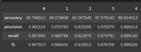
We calculate some metrics such as accuracy, recall, prediction and f1-score.
					from sklearn.metrics import accuracy_score, precision_recall_fscore_support

def calculate_results(y_true, y_pred):
"""
Calculates model accuracy, precision, recall and f1 score of a binary classification model.

Args:
y_true: true labels in the form of a 1D array
y_pred: predicted labels in the form of a 1D array

Returns a dictionary of accuracy, precision, recall, f1-score.
"""


  # Calculate model accuracy
  model_accuracy = accuracy_score(y_true, y_pred) * 100
  # Calculate model precision, recall and f1 score using "weighted average
  model_precision, model_recall, model_f1, _ = precision_recall_fscore_support(y_true, y_pred, average="weighted")
  model_results = {"accuracy": model_accuracy,
                  "precision": model_precision,
                  "recall": model_recall,
                  "f1": model_f1}
  return model_results

def combine_results(y_true, y_pred):
results = {}
for index in range(num_classes):
results[f'{index}'] = calculate_results(y_true=test_dict[f'{index}'], y_pred=model_1_preds[f'{index}'])
return results
And finally, output them in a Panda dataframe.
					import pandas as pd
results= combine_results(y_true=test_dict, y_pred=model_1_preds)
pd.DataFrame(results)
For any questions, reach out to me.

This is a great job!
Dear Lejdi ,
Your CNN model for smart contracts vulnerability looks great model.
Please , I would like you to develop a hybrid GRU-SVM model to identify vulnerabilities in Ethereum smart contracts using the same datasets from https://huggingface.co/datasets/mwritescode/slither-audited-smart-contracts or any publicly available datasets.
Thank you.