
Home » House Price Prediction using Machine Learning
House Price Prediction using Machine Learning

Introduction
In this article, we will go and practice what we’ve learned from the previous article on Linear Regression. We will try to predict the best the house prices using different techniques in Machine Learning. This hands-on guide about house price prediction using Machine Learning is developed in Kaggle and you need to create a Kaggle account to get access to the dataset we are going to use. I would encourage you to join the competition and at the end of this guide, submit a prediction and check how you will rank among other Machine Learning developers.
Take a cup of coffee, and follow along.
At the end of this guide, you will learn:
- What is feature engineering?
- Why is it important to create new features?
- How to optimize model’s hyperparameters?
Table of Contents
Data Collection
First of all, we are going to start by exploring our data and get to know them better. One of the most important aspects in Machine Learning is to understand the data as much as possible. In the following block of code, we are loading from the specified path the training data and displaying the top rows.
					import pandas as pd
train_df = pd.read_csv("/kaggle/input/house-prices-advanced-regression-techniques/train.csv")
train_df.head()
Our data consists of 81 columns, among which we can find the Id and the SalePrice. SalePrice is the target we are going to predict.
Since the target data is continuous, meaning it can take any numerical value within a range, we know that we are working with a regression problem. On the other hand, had it been a discrete number, meaning it can only take distinct values like 0 or 1, the problem would have been one of classification.
Great! That’s what happens when you start looking at the data. You start analyzing and step-by-step you take small decisions.
					Index(['Id', 'MSSubClass', 'MSZoning', 'LotFrontage', 'LotArea', 'Street',
       'Alley', 'LotShape', 'LandContour', 'Utilities', 'LotConfig',
       'LandSlope', 'Neighborhood', 'Condition1', 'Condition2', 'BldgType',
       'HouseStyle', 'OverallQual', 'OverallCond', 'YearBuilt', 'YearRemodAdd',
       'RoofStyle', 'RoofMatl', 'Exterior1st', 'Exterior2nd', 'MasVnrType',
       'MasVnrArea', 'ExterQual', 'ExterCond', 'Foundation', 'BsmtQual',
       'BsmtCond', 'BsmtExposure', 'BsmtFinType1', 'BsmtFinSF1',
       'BsmtFinType2', 'BsmtFinSF2', 'BsmtUnfSF', 'TotalBsmtSF', 'Heating',
       'HeatingQC', 'CentralAir', 'Electrical', '1stFlrSF', '2ndFlrSF',
       'LowQualFinSF', 'GrLivArea', 'BsmtFullBath', 'BsmtHalfBath', 'FullBath',
       'HalfBath', 'BedroomAbvGr', 'KitchenAbvGr', 'KitchenQual',
       'TotRmsAbvGrd', 'Functional', 'Fireplaces', 'FireplaceQu', 'GarageType',
       'GarageYrBlt', 'GarageFinish', 'GarageCars', 'GarageArea', 'GarageQual',
       'GarageCond', 'PavedDrive', 'WoodDeckSF', 'OpenPorchSF',
       'EnclosedPorch', '3SsnPorch', 'ScreenPorch', 'PoolArea', 'PoolQC',
       'Fence', 'MiscFeature', 'MiscVal', 'MoSold', 'YrSold', 'SaleType',
       'SaleCondition', 'SalePrice'],
      dtype='object')
Data Analysis
The next process on the line is data analysis. We aim at understanding what type of features are we dealing with. Let’s make some questions.
- Are they all continuous?
- Do we have categorical features?
- Are there null values?
- How are we going to encode the categorical features?
In order to answer the first two questions, let’s execute the following block of code.
					discrete_features = train_df.select_dtypes(include=['int', 'float'])
categorical_features = train_df.select_dtypes(include=['object'])

print(f'Discrete features are: {discrete_features.columns}\n\n Categorical features are: {categorical_features.columns}')
And this is what we get. There are 38 discrete features and 43 categorical features.
					Discrete features are: Index(['Id', 'MSSubClass', 'LotFrontage', 'LotArea', 'OverallQual',
       'OverallCond', 'YearBuilt', 'YearRemodAdd', 'MasVnrArea', 'BsmtFinSF1',
       'BsmtFinSF2', 'BsmtUnfSF', 'TotalBsmtSF', '1stFlrSF', '2ndFlrSF',
       'LowQualFinSF', 'GrLivArea', 'BsmtFullBath', 'BsmtHalfBath', 'FullBath',
       'HalfBath', 'BedroomAbvGr', 'KitchenAbvGr', 'TotRmsAbvGrd',
       'Fireplaces', 'GarageYrBlt', 'GarageCars', 'GarageArea', 'WoodDeckSF',
       'OpenPorchSF', 'EnclosedPorch', '3SsnPorch', 'ScreenPorch', 'PoolArea',
       'MiscVal', 'MoSold', 'YrSold', 'SalePrice'],
      dtype='object')

 Categorical features are: Index(['MSZoning', 'Street', 'Alley', 'LotShape', 'LandContour', 'Utilities',
       'LotConfig', 'LandSlope', 'Neighborhood', 'Condition1', 'Condition2',
       'BldgType', 'HouseStyle', 'RoofStyle', 'RoofMatl', 'Exterior1st',
       'Exterior2nd', 'MasVnrType', 'ExterQual', 'ExterCond', 'Foundation',
       'BsmtQual', 'BsmtCond', 'BsmtExposure', 'BsmtFinType1', 'BsmtFinType2',
       'Heating', 'HeatingQC', 'CentralAir', 'Electrical', 'KitchenQual',
       'Functional', 'FireplaceQu', 'GarageType', 'GarageFinish', 'GarageQual',
       'GarageCond', 'PavedDrive', 'PoolQC', 'Fence', 'MiscFeature',
       'SaleType', 'SaleCondition'],
      dtype='object')
Now, let’s check if we are dealing with any columns that contains null values. If yes, let’s find which are those columns.
					# Columns that contain null values
columns_with_null_values = train_df.columns[train_df.isnull().any()]
columns_with_null_values
The result that we get is as follows. There are 19 columns that contain at least one NaN value. When we come to this conclusion, we have to take another important decision. What are we going to do about these NaN values? Before we go to that, let’s understand which of these features are categorical and which are discrete.
					Index(['LotFrontage', 'Alley', 'MasVnrType', 'MasVnrArea', 'BsmtQual',
       'BsmtCond', 'BsmtExposure', 'BsmtFinType1', 'BsmtFinType2',
       'Electrical', 'FireplaceQu', 'GarageType', 'GarageYrBlt',
       'GarageFinish', 'GarageQual', 'GarageCond', 'PoolQC', 'Fence',
       'MiscFeature'],
      dtype='object')
To do that we will execute the following code block, the result of which let us know that both discrete and categorical features contain NaN values.
					columns_with_null_values = train_df.columns[train_df.isnull().any()]

discrete_features_with_nulls = [col for col in columns_with_null_values if pd.api.types.is_float_dtype(train_df[col])]
categorical_features_with_nulls = [col for col in columns_with_null_values if pd.api.types.is_object_dtype(train_df[col])]

print(f"Discrete features that contain null values are: {discrete_features_with_nulls}")
print(f"Categorical features that contain null values are: {categorical_features_with_nulls}")
					Discrete features that contain null values are: ['LotFrontage', 'MasVnrArea', 'GarageYrBlt']
Categorical features that contain null values are: ['Alley', 'MasVnrType', 'BsmtQual',
'BsmtCond', 'BsmtExposure', 'BsmtFinType1', 'BsmtFinType2', 'Electrical',
'FireplaceQu', 'GarageType', 'GarageFinish', 'GarageQual', 'GarageCond',
'PoolQC', 'Fence', 'MiscFeature']
Data Cleaning & Correcting
In this step, we are going to look at how we should clean and correct our data before feeding them to our model.
Values might be missing for different reasons. However, it might be the case that they follow a pattern. There are three types of missing values:
- Missing At Random (MAR)
- The reason for missing values can be explained by variables on which we have complete information.
- There is some relationship between the missing data and other values/data.
- Missing Completely At Random (MCAR)
- The probability of data missing is the same for all the observations.
- There is no pattern.
- Missing Not At Random (MNAR)
- Missing values depend on the unobserved data.
- There is some structure/pattern in missing data and other observed data can not explain it.
It’s critical to manage the missing values correctly. If there are missing values in the dataset, a lot of machine learning algorithms perform poorly. Nonetheless, data with missing values is supported by algorithms such as K-nearest and Naive Bayes. Incorrect results could arise from developing a biased machine learning model if the missing values are not appropriately handled.
Deleting the missing values
This approach is very quick and dirty, but it is not recommended. The reason behind it is that you might end up deleting useful data from the dataset. Values might be missing not at a random pattern (MNAR) and therefore, you will get rid of this information from your dataset.
If the missing values are missing at random (MAR) or completely at random (MCAR), then they can be deleted.
Imputing the missing values
The technique of substituting values for missing data is known as imputation. It is referred to as “unit imputation” when a data point is substituted, and “item imputation” when a data point’s component is substituted. Three primary issues arise when data is missing: significant bias can be introduced, processing and interpretation of the data becomes more difficult, and efficiency is reduced.
Hands-On Data Cleaning & Correcting
Let’s try to understand the pattern of the missing values.
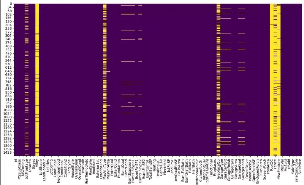
					import seaborn as sns
import matplotlib.pyplot as plt

plt.figure(figsize=(15,8))
sns.heatmap(df.isnull(), cbar=False, cmap='viridis')
plt.show()
Great! Let’s analyze the following heatmap. As we can see, the Alley contains mostly NaN values, same as MasVnrType, PoolQC, MiscFeature and Fence.
However, in the data description it is written that a NaN in Alley/Fence means that there is no alley access/no fence, respectively. Furthermore, a NaN in PoolQC means there is no pool. This feature is correlated with PoolArea. Where we see a PoolArea value of 0, there is a PoolQC of NaN.
On the other hand, FireplaceQu contains NaN values when the Fireplaces value for the respective row is 0. And that makes sense. You can’t provide a quality metric for something you don’t have.
Furthermore, the NaN values in the column named MasVnrType stands for None. If there is no garage (GarageType is NaN), then the other metrics (GarageYrBlt, GarageFinish, GarageQual, GarageCond) about the garage will be NaN as well.
Nonetheless, there is something fishy. Whenever the MasVnrType is NaN, the column MasVnrArea not always contains the value 0. That is something we need to fix.
LotFrontage is the linear feet of street connected to property. It refers to the total length of the street or road that directly borders or is connected to a specific property. It is a measurement of the amount of street frontage that the property has. This measurement is often relevant in real estate, as it can impact the property’s accessibility, visibility, and sometimes its value. In our case, it contains null values that we need to understand why. I suspect that it is missing information that must be filled in a form.
We see that when there is no basement, the other properties about the basement contain NaN values. However, there is one entry that contains NaN in the BsmtExposure column when the BsmtQual and BsmtCondare other than NaN. I suspect that this basement has no exposure, and that’s why it is left as NaN.
Null Values Handling
Based on the analysis we made above, now we will focus on filling the missing values in the most appropriate way.
For LotFrontage, we will use the average LotFrontage within each MsZoning group.
For GarageYrBuilt, we will use the year the house was built. Normally, when you build a house, you build also the garage.
For categorical features, we need to transform and encode them into numbers. NaN values will be first filled with a value like None and then encoded to numbers.
					# Add a value of 0 whenever there is a null value in the MasVnrType column
train_df.loc[train_df['MasVnrType'].isna(), 'MasVnrArea'] = 0

# Calculate the average LotFrontage within each MSZoning group
average_lot_frontage = train_df.groupby('MSZoning')['LotFrontage'].transform('mean')

# Fill null values in LotFrontage with the group-wise averages
train_df['LotFrontage'] = train_df['LotFrontage'].fillna(average_lot_frontage)

# Add a value of No whenever there is a null value in the BsmtExposure column
condition = (train_df['BsmtCond'].notna()) & (train_df['BsmtExposure'].isna())
train_df.loc[condition, 'BsmtExposure'] = 'No'

# Give a value of FuseF to null row in Electrical because based on the SalePrice, it is a fair amount for a FuseF
train_df.loc[train_df['Electrical'].isna(), 'Electrical'] = 'FuseF'

train_df['BsmtQual'].fillna('None', inplace=True)

train_df['BsmtQual'].fillna('None', inplace=True)
train_df['BsmtCond'].fillna('None', inplace=True)
train_df['BsmtExposure'].fillna('None', inplace=True)
train_df['BsmtFinType1'].fillna('None', inplace=True)
train_df['BsmtFinType2'].fillna('None', inplace=True)
train_df['FireplaceQu'].fillna('None', inplace=True)
train_df['GarageFinish'].fillna('None', inplace=True)
train_df['GarageQual'].fillna('None', inplace=True)
train_df['GarageCond'].fillna('None', inplace=True)
train_df['PoolQC'].fillna('None', inplace=True)
train_df['Fence'].fillna('None', inplace=True)

# If the value of the garage built is missing, add that of the year the house was built
train_df['GarageYrBlt'].fillna(train_df['YearBuilt'], inplace=True)
Categorical Feature Encoding
It refers to the process of converting categorical or textual data into numerical format, so that it can be used as input for algorithms to process. The reason for encoding is that most machine learning algorithms work with numbers and not with text or categorical variables.
There are multiple techniques for categorical feature encoding.
- One-Hot Encoding
- A binary column is created for each unique category in the variable.
- If the category is present, the corresponding column is set to 1. All other columns are set to 0, and vice versa.
- Label Encoding
- Each unique category is assigned a unique integer value.
- One of the drawbacks this method has is that it could create bias. The assigned integers may be misinterpreted by the machine learning algorithm as having an ordered relationship when in fact they do not.
- Ordinal Encoding
- It is used when the categories in a variable has a natural ordering.
- The categories are assigned a numerical value based on their order, such as 1, 2, 3, etc.
- Binary Encoding
- Instead of creating a separate column for each category, the categories are represented as binary digits.
- Count Encoding
- It is a method for encoding categorical variables by counting the number of times a category appears in the dataset.
- Target Encoding
- The average target value for each category is calculated and this average value is used to replace the categorical feature.
Hands-On Feature Encoding
In our case, we will use a mixture of TargetEncoding, LabelEncoding and OrdinalEncoding. We will use the OrdinalEncoding where there is an order.
I have encoded more labels with ordinal encoding and you can view them in the code published on Kaggle.
					from sklearn.preprocessing import LabelEncoder, OrdinalEncoder
from category_encoders import TargetEncoder

bsmt_qual_ordered_categories =[['None', 'Po', 'Fa', 'TA', 'Gd', 'Ex']]
ordinal_encoder = OrdinalEncoder(categories=bsmt_qual_ordered_categories)
train_df['BsmtQual'] = ordinal_encoder.fit_transform(train_df[['BsmtQual']])
train_df['BsmtCond'] = ordinal_encoder.fit_transform(train_df[['BsmtCond']])

bsmt_exposure_ordered_categories =[['None','No', 'Mn', 'Av', 'Gd']]
ordinal_encoder = OrdinalEncoder(categories=bsmt_exposure_ordered_categories)
train_df['BsmtExposure'] = ordinal_encoder.fit_transform(train_df[['BsmtExposure']])

bsmt_fin_type_1_categories = [['None','Unf', 'LwQ', 'Rec', 'BLQ', 'ALQ', 'GLQ']]
ordinal_encoder = OrdinalEncoder(categories = bsmt_fin_type_1_categories)
train_df['BsmtFinType1'] = ordinal_encoder.fit_transform(train_df[['BsmtFinType1']])
train_df['BsmtFinType2'] = ordinal_encoder.fit_transform(train_df[['BsmtFinType2']])

# Use target encoder for the rest of the features based on OverallQual
target_encoder = TargetEncoder()
for colname in train_df.select_dtypes(include=["object"]):
    train_df[colname] =  target_encoder.fit_transform(train_df[[colname]], train_df['OverallQual'])
Features and Targets Definition
Let’s define the X which represents the features and the y which represents the target for our dataset.
					y = train_df['SalePrice']
X = train_df.drop(columns=['Id', 'SalePrice'])
Feature Importance
Let’s evaluate the importance of each discrete feature, and how much it will contribute to our model. The code below calculates mutual information for a continuous target variable.
					from sklearn.feature_selection import mutual_info_regression

def make_mi_scores(X, y, discrete_features):
    mi_scores = mutual_info_regression(X, y, discrete_features=discrete_features)
    mi_scores = pd.Series(mi_scores, name="MI Scores", index=X.columns)
    mi_scores = mi_scores.sort_values(ascending=True)
    return mi_scores

discrete_features_X = X.dtypes == int
mi_scores = make_mi_scores(X, y, discrete_features_X)

import matplotlib.pyplot as plt
def plot_mi_scores(scores):
    scores = scores.sort_values(ascending=True)
    width = np.arange(len(scores))
    ticks = list(scores.index)
    plt.barh(width, scores)
    plt.yticks(width, ticks)
    plt.title("Mutual Information Scores")


plt.figure(dpi=100, figsize=(15, 15))
plot_mi_scores(mi_scores)
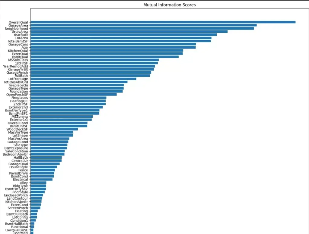
Let’s draw a couple of conclusions from the plot we see above. First of all, OverallQual provides the most information and we can use it develop other features based on that.
MiscFeatures does not add any important information, as well as Utilities , Street, PoolArea and MiscVal. We need to analyze these features better in order to develop new features that use them and provide better information.
Model Baseline
Whenever you want to solve a problem using Machine Learning, you need to have a baseline for your model. Remember, you cannot improve what you can’t measure.
First, we will define the scorer that is the function that evaluates the error of our model’s predictions. We will use the root mean squared error.
					def root_mean_squared_error(targets, predictions):
    return np.sqrt(((np.log(predictions) - np.log(targets)) ** 2).mean())

from sklearn.metrics import make_scorer
scorer = make_scorer(score_func=root_mean_squared_error)
Great! It’s time to create our baseline model. We will use the RandomForestRegressor and evaluate the baseline using cross_val_score.
What is the cross_val_score? It is a function that splits the dataset into x folds. It trains the model in x-1 folds and finally, evaluates it in the 1 fold.
					from sklearn.ensemble import RandomForestRegressor
baseline = RandomForestRegressor()
baseline_score = cross_val_score(
    baseline, X, y, cv=5, scoring=scorer
)
baseline_score = baseline_score.mean()

print(f"RMSE Baseline Score: {baseline_score}")

# My output => RMSE Baseline Score: 0.14376049335800697
Feature Engineering
Feature engineering is the process of creating new features or modifying existing ones in a dataset to improve the performance of a machine learning model. The goal is to enhance the model’s ability to learn patterns and make accurate predictions. Effective feature engineering can significantly impact the success of a machine learning model, often more than the choice of the algorithm.
Let’s create a new feature! Since we have the year the house was built and the year it was sold, we can calculate the age of the property. I expect that the newly built properties are sold for more than the old ones.
train_df['Age'] = train_df['YrSold'] - train_df['YearBuilt']
Great! Your first feature engineered by you.
Next steps
Now, you should try to improve your baseline. You could experiment with our models and create new features as we did above.
If you want to learn more, go to this notebook on Kaggle.
If you learned something from this article, consider supporting by sharing or donating.
